
 Buch kaufen
 Buch kaufen
 Buch kaufen
Nächstes Kapitel: Erzeugen von synthetischen Testdaten mit Python
Andere verfügbaren Datensätze
Scikit-learn stellt eine Vielzahl von Datensätzen zum Testen von Lernalgorithmen zur Verfügung.
Sie kommen in drei Geschmacksrichtungen:
- Gepackte Daten: Diese kleinen Datensätze sind Teil der Installation von scikit-learn
- Herunterladbare Daten: Diese größeren Datensätze stehen zum Download zur Verfügung und können per Scikit gelernt werden
Enthält Tools, die diesen Prozess optimieren. Diese Tools finden Sie in
sklearn.datasets.fetch_ * - Generierbare Daten: Es gibt mehrere Datensätze, die auf Modellen basieren und mittels
seed-Werten generiert werden können auf a generiert werden können. Diese sind alssklearn.datasets.make_ *verfügbar
Mittels der Tab-Vervollständigungsfunktion von IPython können Sie die verfügbaren Dataset Loader, Fetcher und Generatoren nach dem Import des datasets Submoduls aus sklearn untersuchen,
datasets.load_<TAB>
or
datasets.fetch_<TAB>
or
datasets.make_<TAB>from sklearn import datasets
Warnung: Viele dieser Datasets sind sehr groß und das Herunterladen kann sehr lange dauern!
Digits-Datenset laden
Wir werden uns nun einen dieser Datensätze genauer ansehen. Wir schauen uns den Ziffern-Datensatz an. Wir laden ihn zuerst:
from sklearn.datasets import load_digits
digits = load_digits()
Wir können uns wieder einen Überblick über die verfügbaren Attribute verschaffen, indem wir uns die "keys" anschauen:
digits.keys()
Werfen wir einen Blick auf die Anzahl der Elemente und Funktionen:
n_samples, n_features = digits.data.shape
print((n_samples, n_features))
print(digits.data[0])
print(digits.target)
Die Daten liegen auch unter digits.images vor. Dabei handelt es sich um die Rohdaten der Bilder in der Form 8 Zeilen und 8 Spalten.
Bei "data" entspricht ein Bild einem eindimensionen Numpy-Array mit der Länge 64, und images enthält 2-dimensionale numpy-Arrays mit der Shape (8, 8)
print("Shape eines Items: ", digits.data[0].shape)
print("Datentype eines Items: ", type(digits.data[0]))
print("Shape eines Items: ", digits.images[0].shape)
print("Datentype eines Items: ", type(digits.images[0]))
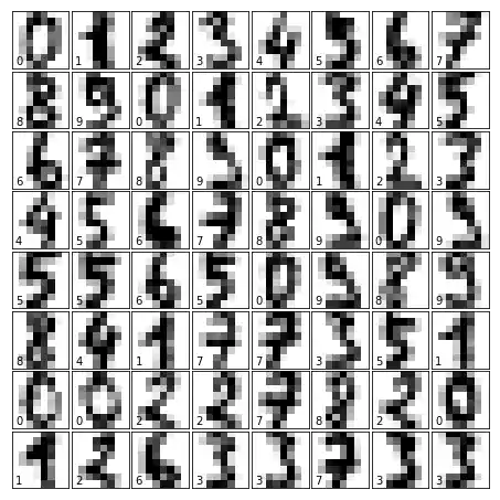
Nun wollen wir die Daten visualisieren:
import matplotlib.pyplot as plt
# set up the figure
fig = plt.figure(figsize=(6, 6))  # figure size in inches
fig.subplots_adjust(left=0, right=1, bottom=0, top=1, hspace=0.05, wspace=0.05)

# plot der Ziffern:
# jedes Bild besteht aus 8x8 Pixel.
for i in range(64):
    ax = fig.add_subplot(8, 8, i + 1, xticks=[], yticks=[])
    ax.imshow(digits.images[i], cmap=plt.cm.binary, interpolation='nearest')

    # label the image with the target value
    ax.text(0, 7, str(digits.target[i]))
Übungen
Aufgabe 1
sklearn enthält einen „Wein-Datensatz“.
- Suchen und laden Sie diesen Datensatz
- Können Sie eine Beschreibung finden?
- Wie heißen die Klassen und die Features?
- Wo sind die Daten und die Daten und die Labels?
Aufgabe 2
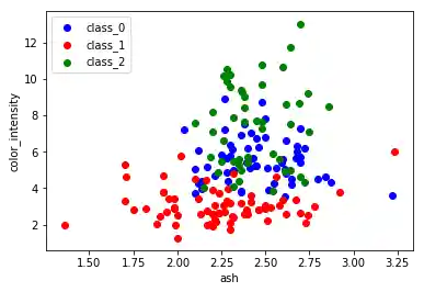
Erzeugen Sie einen scatter-Plot mit den Features ash und color_intensity
des Wine-Datensatzes.
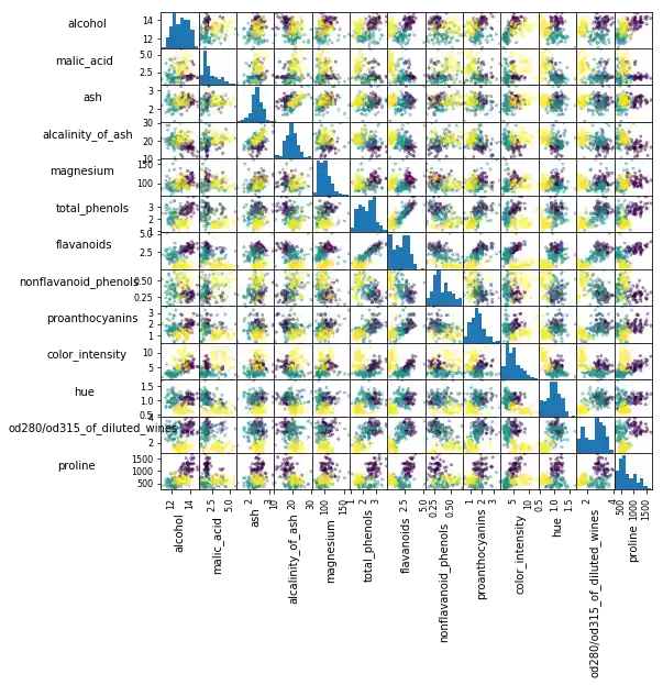
Aufgabe 3
Erzeugen Sie eine Scatter-Matrix für das Wine-Datenset
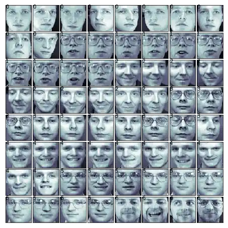
Aufgabe 4
Finden und laden Sie den Olivetti-Datensatz der Photos mit Gesichtern enthält und stellen Sie die Gesichter dar.
from sklearn import datasets

wine = datasets.load_wine()
Die BEschreibung erhält man mittels:
print(wine.DESCR)
Die Namen der Klassen und der Features erhalten wir mit den Attributen "target_names" und "feature_names":
print(wine.target_names)
print(wine.feature_names)
daten = wine.data
gelabelte_daten = wine.target
Lösung zu Aufgabe 2
from sklearn import datasets
import matplotlib.pyplot as plt

wine = datasets.load_wine()

features = 'ash', 'color_intensity'
features_index = [wine.feature_names.index(features[0]),
                  wine.feature_names.index(features[1])]


colors = ['blue', 'red', 'green']

for label, color in zip(range(len(wine.target_names)), colors):
    plt.scatter(wine.data[wine.target==label, features_index[0]],
                wine.data[wine.target==label, features_index[1]],
                label=wine.target_names[label],
                c=color)

plt.xlabel(features[0])
plt.ylabel(features[1])
plt.legend(loc='upper left')
plt.show()
Lösung zu Aufgabe 3
import pandas as pd
from sklearn import datasets
wine = datasets.load_wine()
def rotate_labels(df, axes):
""" changing the rotation of the label output,
y labels horizontal and x labels vertical """
n = len(df.columns)
for x in range(n):
for y in range(n):
# to get the axis of subplots
ax = axs[x, y]
# to make x axis name vertical
ax.xaxis.label.set_rotation(90)
# to make y axis name horizontal
ax.yaxis.label.set_rotation(0)
# to make sure y axis names are outside the plot area
ax.yaxis.labelpad = 50
wine_df = pd.DataFrame(wine.data, columns=wine.feature_names)
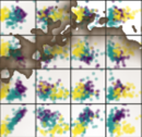
axs = pd.plotting.scatter_matrix(wine_df,
c=wine.target,
figsize=(8, 8),
);
rotate_labels(wine_df, axs)
Lösung zur Aufgabe 4
from sklearn.datasets import fetch_olivetti_faces
# Laden des Datensatzes
faces = fetch_olivetti_faces()
faces.keys()
n_samples, n_features = faces.data.shape
print((n_samples, n_features))
np.sqrt(4096)
faces.images.shape
faces.data.shape
print(np.all(faces.images.reshape((400, 4096)) == faces.data))
# set up the figure
fig = plt.figure(figsize=(6, 6))  # figure size in inches
fig.subplots_adjust(left=0, right=1, bottom=0, top=1, hspace=0.05, wspace=0.05)

# plot the digits: each image is 8x8 pixels
for i in range(64):
    ax = fig.add_subplot(8, 8, i + 1, xticks=[], yticks=[])
    ax.imshow(faces.images[i], cmap=plt.cm.bone, interpolation='nearest')

    # label the image with the target value
    ax.text(0, 7, str(faces.target[i]))
Weitere Datensätze
sklearn verfügt über viele weitere Datensätze. Wenn Sie noch weitere benötigen, finden Sie mehr in dieser interessanten Liste von Datensätzen bei Wikipedia.
Nächstes Kapitel: Erzeugen von synthetischen Testdaten mit Python